Hide Zeros in Excel
Before going ahead with the steps to Hide Zeros in Excel, you may want to understand the difference between hiding zeros and removing zeros in Excel. When you hide zeros in Excel, you are only hiding the data in cells containing zero values, the cells continue to retain their zero values data. This practically means that the data (zero value) in the cell will be considered in all calculations and formulas. In comparison, when you remove zeros from an Excel Data field, the cell becomes blank and its won’t be considered in formulas and calculations. With this understanding, let us go ahead and take a look at different methods to Hide Zeros in Excel.
1. Automatically Hide Zeros in Excel
Follow the steps below to automatically hide zeros in Excel.
Open the Excel worksheet in which you want to hide zeros and click on the File tab.
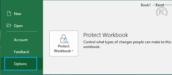
In the File Menu, scroll down to the bottom and click on Options.
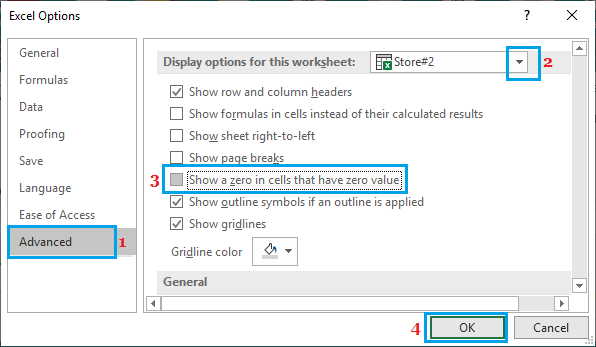
On Excel Options screen, click on Advanced in the left pane. In the right-pane, scroll down to ‘Display options for this worksheet’ section > select the worksheet in which you want to hide zero values and uncheck Show a zero in cells that have zero value option.
Click on OK to save this setting for the worksheet. Once you click on OK, all the cells in the data field having zeros will appear blank.
2. Hide Zeros in Excel Using Conditional Formatting
The above method hides zero values in the entire worksheet and cannot be used to Hide Zeros in a specific range in the data. If you want to hide Zeros in a selected portion of the data, you can use conditional formatting.
Select the Portion of Data in which you want to Hide Zero Values.
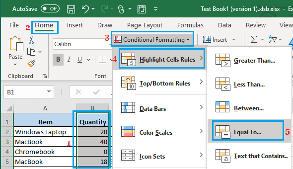
Click on the Home tab > Conditional Formatting > Highlight Cells Rules and click on Equal to option.
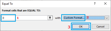
In ‘Equal To’ dialog box, enter 0 in the left field. In the right-field, select Custom Format option and click on OK .
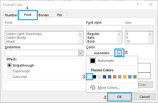
On Format Cells screen, select the Font tab > use the Color drop-down and select white colour.
Click OK to save this setting. The above method hides zeros in Excel by changing the font colour of the cells that have zeros in them to white, which make these cells look blank.
3. Hide Zeros In Excel Using Background Colour
The above method to hide zeros in Excel by changing the font colour to white does not work if the cells in the worksheet have a coloured background. If you have a worksheet with coloured background, you can still hide zero values by following the steps below.
Select the Portion of Data in which you want to Hide Zero Values.
Click on the Home tab > Conditional Formatting > Highlight Cells Rules and click on Equal to option.
In ‘Equal To’ dialog box, enter 0 in the left field. In the right-field, select Custom Format option and click on OK.
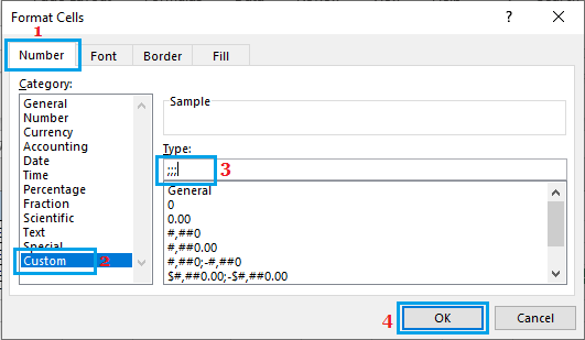
In ‘Format Cells’ screen, click on the Number tab and select Custom option in the left pane. In the right-pane, enter ;;; (3 semi-colons) in the ‘Type’ field and click on OK.
When you apply ;;; (3 semi-colons) format in Excel, it hides both numeric and text values in the cells in which this format is applied. In this case, we are using conditional formatting to applying the 3 semi-colons format only to cells with 0 values.
How to Hide Cells, Rows and Columns In Excel How to Hide Formulas in Excel